Abstract (Note *)
The Phillips curve refers to a negative (or inverse) relationship between unemployment and inflation in an economy—when unemployment is high, inflation tends to be low, and vice versa. This inflation-unemployment link has been observed in many countries during many times, most famously by William Phillips in 1958 looking at historical data for the United Kingdom. If this relationship is stable (or “structural”)—meaning that it holds regardless of changes in the economic environment, including policy adjustment—then policymakers might be able to trade off increases in inflation to achieve lower unemployment, or the inverse.
However, research over the past 40 years has thrown a great deal of doubt onto whether a stable Phillips curve relationship exists. Economists have documented large changes over time in the relationship between unemployment and inflation. In addition, theoretical work has shown that the existence of an empirical association does not necessarily mean that policymakers can exploit that relationship; there may be a statistical correlation—but not a causal link—between inflation and unemployment.
In this essay, we revisit the stability of the Phillips curve. Our key insight is that if the analysis incorporates a central bank seeking to stabilize inflation, national data are likely to provide little information about the existence (or absence) of a stable relationship. We show that regional data can overcome this obstacle. While estimates of Phillips curves using national U.S. data are highly unstable over the past 40 years, we find that estimates based on regional data are remarkably stable. Our results suggest that a 1-percentage-point-lower unemployment rate is associated with higher inflation of 0.3 percentage points over the next year, and the stability of the relationship suggests that it might provide a viable tool for policymakers.
Introduction
The Federal Reserve has been given a dual mandate by Congress in its conduct of monetary policy: Pursue price stability and maximum employment. Similar inflation and employment goals are common among central banks worldwide. On the price stability mandate, the performance of the Federal Reserve since the early 1990s has been remarkably successful. Over the past 20 years, U.S. inflation has averaged 1.9 percent per year, with a maximum 12-month rate of 4.2 percent and a minimum of -1.2 percent. If food and energy components (typically quite volatile) are excluded, inflation has run between 1 percent and 2.9 percent throughout this period.
That central banks can play a central role in affecting prices is widely accepted, but whether monetary policy has a reliable influence on employment is much more controversial. Work on the relationship between inflation and unemployment dates back to Irving Fisher in 1926, who documented a statistical relationship using data from the United States. The topic attracted much more attention when William Phillips published research in 1958 showing a negative relationship between unemployment and the growth rate of nominal wages—the Phillips curve.
The importance of this relationship for the design of monetary policy is clear: If the relationship between unemployment and inflation is structural (meaning it is stable regardless of changes in the economic environment, such as changes in monetary policy), it justifies active monetary policy that reduces some fluctuations in employment and provides a tool by which the Federal Reserve can pursue its employment mandate.
We emphasize if because there has been considerable debate over the past 40 years over whether the Phillips curve relationship is truly structural. Research against this claim includes the fact that estimates of the relationship between unemployment and inflation are sensitive to the time period and monetary policy regime. For example, the relationship in postwar U.S. data changes substantially depending on the period analyzed (see, for example, Atkeson and Ohanian 2001, and Fisher, Liu and Zhou 2002).
In addition, the approach to monetary policy also appears to have changed substantially. For example, when unemployment and inflation both rose dramatically during the 1970s, Federal Reserve Chair Paul Volcker instituted a new policy regime calling for substantial interest rate hikes, resulting in a decline in inflation.
On the theoretical side, research has shown that observed relationships in the data do not imply stable, exploitable relationships by policymakers. In a highly influential 1972 paper, Robert Lucas argued that because people are aware of policy changes, any such changes will affect their expectations for the future. If a central bank changes its policy, therefore, firms and households may well adjust their economic behavior, thereby disrupting observed past relationships in the data (and possibly rendering ineffective the newly implemented policy).
This policy paper makes two central points.
- First, we show that including a central bank that aims to stabilize inflation into the analysis has dramatic implications for understanding the Phillips curve. It implies that national data on inflation and unemployment provide little information about whether a structural relationship exists. In fact, our theory predicts that the relationship will appear unstable as policy goals change, even if a structural relationship exists.
- Second, we show that a remarkably stable relationship between unemployment and inflation emerges when regional, rather than national, data are analyzed, because less-aggregated data allow the analysis to address complications raised by changes in monetary policy. Our results show that a 1-percentage-point-lower unemployment rate is associated with a higher inflation rate of roughly 0.3 percentage points over the next year. The stability of this relationship suggests that it might indeed be exploitable by policymakers.
Instability of the U.S. Phillips curve
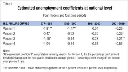
The relationship between inflation and unemployment over the past 40 years has not been stable in the United States in the sense that it varies widely depending on the time period analyzed. The standard procedure for examining this relationship is a statistical analysis of the relationship between current unemployment and future inflation. Researchers use many different formulations of the Phillips curve, varying by the specific data and functional forms used and the time horizon. In Table 1, we report the estimated unemployment coefficient—meaning the amount by which future inflation is predicted to change given a specific change in current employment—of four typical versions over four different time periods. Specifics can be found in Fitzgerald and Nicolini (2013).
Note that the coefficient for each version is substantially different in each time period. For example, in Version 1, the 1977-1984 coefficient found in national data is -1.81, which in this version means that a 1-percentage-point decline in the current unemployment rate is associated with a 1.81-percentage-point increase in future inflation. But the coefficient is near zero in the 1990s (0.04) and during the 2000s (-0.26). This unemployment and future inflation relationship varies substantially across time periods for each version of our Phillips curve. That is, for a variety of standard formulations, there is no apparent structural or stable Phillips curve relationship—a statistical association that appears strong one decade may be weak the next.
A simple theory of monetary policy
To see why this variability by time period exists, we examine the implication of incorporating central bank policy for the observed behavior of inflation and its relationship to unemployment. In particular, we ask whether aggregate data generated by an economy where the central bank uses policy to stabilize inflation can be fruitfully used to learn about any structural relationship between inflation and unemployment. We argue that the answer is no.
Imagine a case where the central bank is concerned about price stability only and sets monetary policy to achieve a specific target rate of annual inflation of, say, 2 percent per year. Suppose also that future inflation depends on current unemployment, as the Phillips curve notion suggests, but also on monetary policy and on other macroeconomic variables and unexpected events, or “shocks.”
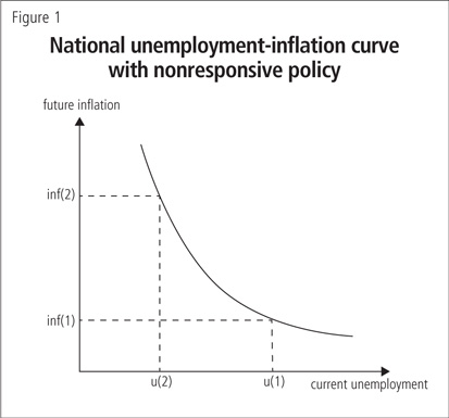
To illustrate our point graphically, first consider what happens if policy does not respond to changes in current data in an attempt to stabilize inflation. This is shown in Figure 1, where current unemployment is shown on the horizontal axis and future inflation on the vertical axis. The downward sloping curve represents the relationship between current unemployment and future inflation, given values for other variables, such as current inflation, and given policy variables, such as the federal funds rate.
In this formulation, policy does not respond in a systematic fashion to observed unemployment or inflation, meaning that policymakers don’t change monetary policy in reaction to observed data. Over time, then, there would be a clear, negative structural relationship, as shown in Figure 1. In this case, every time unemployment is u(1), the average value of inflation in the next period will be inf(1), and every time unemployment is u(2), the average value of future inflation will be inf(2).
What impact will there be on this relationship if we incorporate central bank responses to a Phillips curve trade-off?
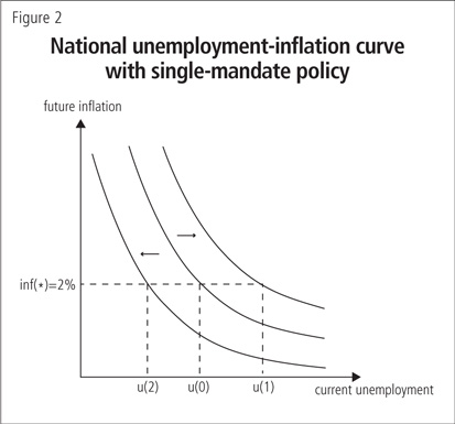
Again, assume that the central bank cares about stabilizing annual inflation at 2 percent (leaving aside, for now, the Fed’s “maximum employment” mandate). The central bank observes the current unemployment rate, and it understands the Phillips curve relationship illustrated in Figure 1. In addition, it knows this inflation-unemployment trade-off can be used to achieve its inflation target. By setting an expansionary monetary policy, it can shift the curve outward—meaning that by changing interest rates, the central bank can achieve its future inflation target despite higher unemployment. Alternatively, it could set a restrictive policy to shift the curve inward, achieving its 2 percent inflation target with lower unemployment.
Thus, if current unemployment is u(1), the central bank will choose policy so as to shift the curve to the right and achieve 2 percent average future inflation, as shown in Figure 2. Similarly, if unemployment is u(2), the central bank will set policy so as to shift the curve to the left and attain average future inflation of 2 percent.
How will inflation behave in this economy? It will, on average, equal 2 percent per year. And the deviations of actual future inflation from 2 percent will be uncorrelated with macroeconomic variables that affect inflation, such as oil price hikes or past inflation. Most crucial to the question addressed in this paper: The current unemployment rate, in particular, will have no correlation with inflation. In sum, data generated by this economy will exhibit no statistical relationship between any of the macroeconomic variables mentioned and future inflation, despite the fact that future inflation is assumed to depend on current unemployment along with other variables.
Why is future inflation uncorrelated with its fundamentals? Because the central bank is following its legislatively set mandate—price stability. It is using policy to keep inflation at 2 percent despite changes in the underlying economy, including movements in the unemployment rate.
According to this theory, the estimated coefficient of the Philips curve should always be zero—that is, there should be no measurable relationship between unemployment and inflation. This stark result reflects the fact that we are considering a central bank with a single mandate. But, in reality, the Federal Reserve has a dual mandate: to stabilize inflation and maximize employment. If a central bank is charged with a dual mandate, the estimated coefficient of the Phillips curve in our theory depends on how much weight it puts on each objective. If it is concerned to any extent about its employment mandate, then the estimated coefficient of the Phillips curve will be negative—a trade-off between inflation and unemployment will exist.
Note a general pattern seen in Table 1. The estimated slope of the Phillips curve is higher for the first subperiod (1977-1984) and goes down (the negative relationship approaches zero) over time. This is consistent with the view that the weight on the employment mandate was high in the 1970s—so there is evidence of a negative Phillips curve using aggregate data—but declined starting with Paul Volcker’s term in 1979—so it became harder to find a negative Phillips curve coefficient in national-level data for the United States. Furthermore, the view that the weight on the employment mandate has fallen is consistent with annual inflation being stabilized pretty tightly around 2 percent over the past 20 years.
Stability of regional Phillips curves
Once an active central bank is incorporated into the analysis, it becomes clear that national data on inflation and unemployment are not useful for exploring whether a structural, or stable, Phillips curve relationship exists. In order to account for the complications raised by incorporating a central bank, we make use of regional data on unemployment and inflation.
We imagine an economy composed of numerous regions and a single central bank. Regional shocks make inflation rates and unemployment rates vary across regions. To simplify, we assume that regions are the same for the most part, but each faces different local disturbances, or shocks.
As before, the central bank aims to stabilize the inflation rate, which, for the central bank, is the average rate over all regions. Policy will therefore move to stabilize average national inflation. Monetary policymakers will react strongly to national shocks that affect inflation in all regions, but react very little to a shock that increases inflation in one region only, since this has little impact on the average. In the absence of central bank response to local conditions, a regional shock that affects unemployment in just a single region can therefore help identify the existence and size of a structural relationship between current labor market conditions and future inflation.
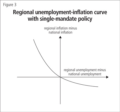
To frame the analysis graphically, consider Figure 3, which plots the regional-national differences for future inflation and current unemployment. Thus, the vertical axis displays the gap between future inflation in a given region and the inflation target set by the central bank; the difference between current unemployment in the same region and average national unemployment is plotted on the horizontal axis.
The curve crosses the origin (where the X axis and Y axis intersect), meaning that future inflation in a region matches the central bank’s national inflation target when unemployment in that region equals the national unemployment figure. The key feature of monetary policy in our theory is that the central bank reacts only when average national inflation rises above or drops below the target; it does not respond to changes in individual regional inflation rates. Thus, in regions where unemployment is lower than the national average, inflation will be higher than the national average and in regions where unemployment is higher than the national average, future inflation will be lower than the national average.
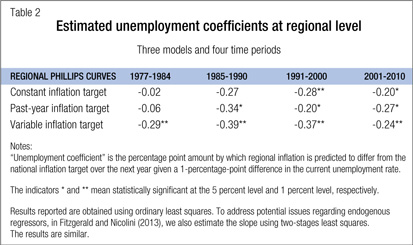
One difficulty with our approach is that we need a measure of the inflation target for the central bank. The Federal Reserve did not provide an explicit inflation target until 2012. To address this issue, we look at three Phillips curve models. In our first model, we assume that the inflation target is constant during the entire period from 1977 onward—clearly an unrealistic assumption since we include the high inflation of the 1970s. In the second model, we assume that the target for the next year is the past year’s inflation rate. In the third model, we include a time period variable, which can be interpreted as a period-by-period estimate of the inflation target.
Table 2 presents our results. Except for the first two numbers in the first column—the period of extremely high unemployment and inflation—the results are remarkable in their consistency. The coefficients across models all have the same interpretation, strongly suggesting a slope around -0.3, with a tight range from -0.39 to -0.20 across models in the final three time periods. These estimates therefore indicate that if unemployment is 1 percentage point higher, inflation over the next year will be 0.3 percentage points lower.
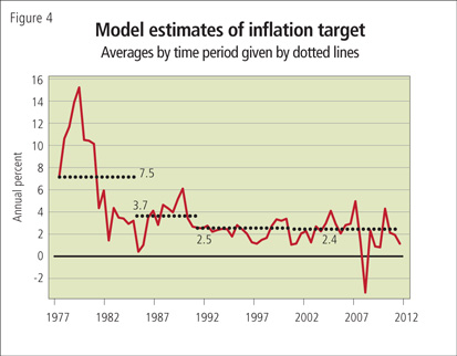
An interesting independent outcome from the third model, with a variable inflation target, is an estimation of the Fed’s implicit inflation target. We plot the estimated values of that target since 1977 to 2010 in Figure 4, together with average values for each for the four subperiods we are considering.
The assumption of a constant or past-year inflation target seems implausible for the 1977-1984 period. We think this also explains why the first two models’ coefficients for the 1977-1984 period are so different from other model and period estimates, and why the model results are so similar over the past 20 years.
Summary
In summary, we argue that the instability of the Phillips curve seen in U.S. data from recent decades is exactly what theory predicts when monetary policymakers pursue a dual mandate while changing emphasis on inflation and unemployment over time. Statistical calculations that use U.S. data on unemployment and inflation provide little evidence as to the underlying relationship between these variables precisely because the central bank is actively seeking to achieve specific policy goals and thereby dampening effects of structural links that may exist.
In contrast, our theory predicts that regional Phillips curve analysis is immune to policy changes made to achieve average national goals. Our data analysis shows that, indeed, the estimates of a Phillips curve trade-off are remarkably stable over the same multidecade period and show a consistent negative relationship between regional unemployment and inflation. This suggests that policymakers may be able to exploit a trade-off between mandates.
Note
* The authors thank Narayana Kocherlakota for asking the question that led to this research and Sam Schulhofer-Wohl for comments. All errors are the authors’.
References
Atkeson, Andrew, and Lee E. Ohanian. 2001. “Are Phillips Curves Useful for Forecasting Inflation?” Federal Reserve Bank of Minneapolis Quarterly Review (Winter): 2-11.
Fisher, Irving. 1926. “A Statistical Relationship Between Unemployment and Price Changes.” International Labor Review 13 (June): 785-92. Reprinted in 1973 as “I Discovered the Phillips Curve.” Journal of Political Economy 81 (March-April): 496-502.
Fisher, Jonas D. M., Te Liu Chin and Ruilin Zhou. 2002. “When Can We Forecast Inflation?” Journal of Economic Perspectives 26 (1): 30-42.
Fitzgerald, Terry, and Juan Pablo Nicolini. 2013. “Is There a Stable Relationship Between Unemployment and Future Inflation? Evidence from U.S. Cities.” Working Paper. Federal Reserve Bank of Minneapolis. Forthcoming.
Lucas, R. E., Jr. 1972. “Expectations and the Neutrality of Money.” Journal of Economic Theory 4: 103-24.
Nicolini, Juan Pablo. 2012. “Monetary Policy and the Quantity Theory of Money.” Mimeo. Federal Reserve Bank of Minneapolis.
Phillips, A. W. 1958. “The Relation Between Unemployment and the Rate of Change of Money Wage Rates in the United Kingdom, 1861-1957.” Economica 25 (100): 283-99.


